O₂graph script
Sometimes it’s helpful to be able to do some quick and dirty data
analysis without having to write python directly. The O₂sclpy package
includes a script called o2graph which is designed to enable quick
analysis with text files or with HDF5 files (especially those
generated by O₂scl). The O2graph script assumes that the
O₂scl library has been installed separately (with HDF5 support
enabled).
Basic usage
The o2graph script is formulated along the same lines as the
acol executable in O₂scl documented at “The acol Command Line Utility”. It operates on one object at a time, and
the basic workflow is the same: read or create an object, manipulate
and/or plot that object, and save the object or the plot to a file.
Similar to acol, the o2graph list of commands and help
screen changes depending on the type of the current object in
memory. Commands common to all types are listed in o2graph --help
or o2graph --commands. Commands applicable to objects of
O₂scl type table are listed by o2graph --commands
table. To obtain the help information on how a particular
command works with a particular type, add the type and the
command as arguments to help, e.g. o2graph --help table plot,
which shows how to plot columns from table objects.
o2graph: A data viewing and processing program for O2scl.
  Version: 0.931

List of command-line options which do not require a current object:

  -addcbar        Add a color bar.
  -alias          Create a command alias.
  -append-images  Combine two images side by side
  -arrow          Plot an arrow.
  -autocorr       Compute autocorrelation coefficients.
  -backend        Select the matplotlib backend to use.
  -bl-import      Load a GLTF file into Blender
  -bl-six-mp4     View each axis of a set of 3D objects in a movie
  -bl-yaw-mp4     View 3D objects in a movie by rotating the camera
  -calc           Compute the value of a constant expression.
  -canvas         Create a plotting canvas.
  -clear          Clear the current object.
  -clf            Clear the current figure.
  -cmap           Create a continuous colormap or list colormaps.
  -colors         Show color information.
  -commands       List available commands for current or specified type.
  -constant       Get or modify a physical or numerical constant.
  -convert        Manipulate or use a unit conversion factor.
  -create         Create an object.
  -docs           Open local O₂scl HTML documentation.
  -download       Download a file from the specified URL.
  -ellipse        Plot an ellipse.
  -error-point    Plot a single point with errorbars.
  -eval           Run the python eval() function.
  -exec           Run the python code specified in a file.
  -exit           Exit (synonymous with 'quit').
  -filelist       List objects in a HDF5 file.
  -generic        Read an object from a generic text file.
  -get            Get the value of a parameter.
  -gltf           Produce a GLTF file with the current set of 3D objects.
  -h5-copy        Copy an O₂scl-generated HDF5 file.
  -help           Show help information.
  -image          Plot a png file in a matplotlib window.
  -inset          Add a new set of axes
  -interactive    Toggle interactive mode.
  -internal       Output current object in the internal HDF5 format.
  -license        Show license information.
  -line           Plot a line from :math:`(x_1,y_1)` to :math:`(x_2,y_2)`
  -modax          Modify current axes properties.
  -mp4            Create an mp4 file from a series of images.
  -nderiv         Numerically differentiate a user-specified function.
  -ninteg         Numerically integrate a user-specified function.
  -no-intro       Do not print introductory text.
  -output         Output the current object to screen or text file.
  -plotv          Plot several vector-like data sets.
  -point          Plot a single point.
  -preview        Preview the current object.
  -python         Begin an interactive python session.
  -quit           Quit (synonymous with 'exit').
  -read           Read an object from an O₂scl-style HDF5 file.
  -rect           Plot a rectangle.
  -run            Run a file containing a list of commands.
  -save           Save the current plot in a file.
  -selax          Select an axis from the current list of axes
  -set            Set the value of a parameter.
  -shell          Run a shell command.
  -show           Show the current plot.
  -slack          Send a slack message.
  -subadj         Adjust spacing of subplots
  -subplots       Create subplots.
  -td-arrow       Create a 3D arrow (experimental)
  -td-axis        Create a 3D axis (experimental).
  -td-axis-label  Create a 3D axis label (experimental).
  -td-cyl         Create a 3D cylinder (experimental)
  -td-den-plot    Create a 3D density plot (experimental).
  -td-icos        Create a 3D icosphere (experimental).
  -td-line        Plot a line in a 3d visualization (experimental)
  -td-mat         Create a 3D material (experimental)
  -td-pgram       Plot a 3D parallelogram (experimental)
  -td-point       Plot a 3D point (experimental)
  -td-scatter     Create a 3D scatter plot (experimental).
  -text           Plot text in the data coordinates.
  -textbox        Plot a box with text.
  -ttext          Plot text in window coordinates [(0,0) to (1,1)].
  -type           Output the type of the current object.
  -version        Print version information and O₂scl settings.
  -warranty       Show warranty information.
  -wdocs          Open remote HTML O₂scl or O₂sclpy docs.
  -xlimits        Set the x-axis limits
  -xml-to-o2      Parse doxygen XML to generate runtime docs.
  -xtitle         Add a title for the x-axis
  -ylimits        Set the y-axis limits
  -yt-ann         Annotate a yt rendering (experimental).
  -yt-arrow       Plot an arrow in a yt volume visualization.
  -yt-axis        Add an axis to the yt volume.
  -yt-box         Create a box in a yt visualization.
  -yt-line        Plot a line in a yt volume visualization.
  -yt-path        Add a path to the yt animation.
  -yt-render      Render the yt volume visualization.
  -yt-source-list List yt sources
  -yt-text        Add text to the yt volume.
  -yt-tf          Edit the yt transfer function.
  -yt-xtitle      Add a title to the x axis in yt
  -yt-ytitle      Add a title to the y axis in yt
  -yt-ztitle      Add a title to the z axis in yt
  -ytitle         Add a title for the y-axis
  -zlimits        Set the z-axis limits

------------------------------------------------------------------------------
Additional help topics: fonts, functions, index-spec, markers, markers-plot,
mult-vector-spec, strings-spec, types, value-spec, and vector-spec.
Integration with O₂scl
The o2graph script implements all of the commands from the
acol executable in O₂scl documented at
“The acol Command Line Utility”
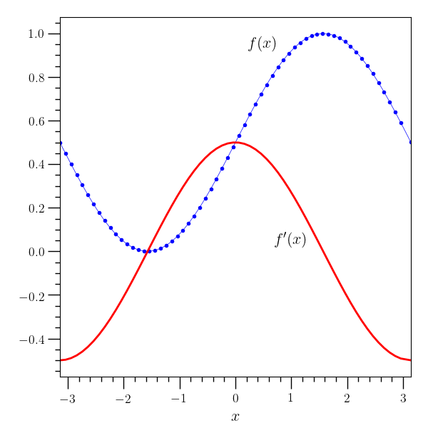
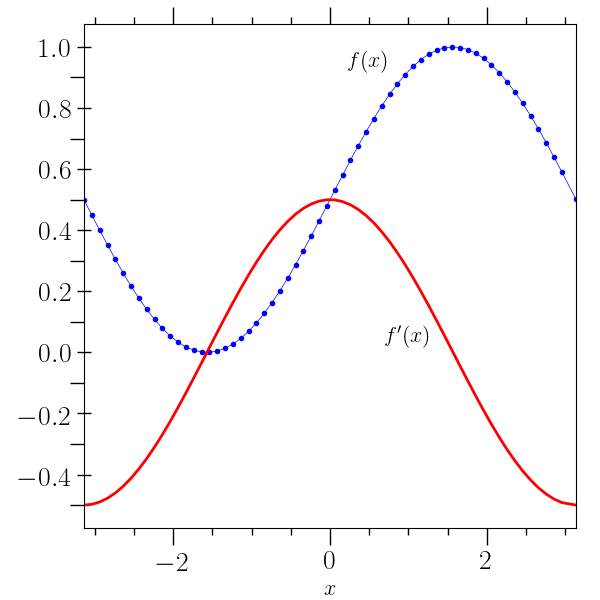
First plot example
# This example creates a simple plot with one independent variable.
# The 'create' command creates an o2scl table object, 'function'
# creates a new column from a function, and 'deriv' creates a new
# column using interpolation to obtain the derivative. The command
# 'output' creates a HDF5 file which stores the full table. Quotes and
# parentheses are used to avoid confusion between negative values and
# commands. Also, in LaTeX strings, and extra space is placed after
# some $'s to avoid confusion with shell variables.
#
o2graph -backend Agg -create table x grid:-3.14,3.14,0.1 \
        -function "(1+sin(x))/2" y \
        -set xlo "(-3.14)" -set xhi 3.14 -xtitle "$ x$" -deriv x y yp \
        -preview 20 -internal data/table_plot.o2 \
        -plot x y marker=.,color=blue \
        -plot x yp lw=2,color=red -text 0.5 0.95 "$ f(x)$" \
        -text 1 0.05 "$ f^{\prime}(x)$" -save figures/table_plot.png
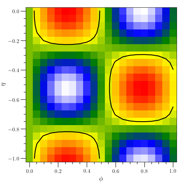
Density plot and contour line example
# This example creates a density plot and overlying contour plot
# with two independent variables.
#
o2graph -create table3d x grid:0,1,0.05 y "grid:(-1),0,0.05" \
        z "sin(x*6)*cos(y*6)" \
        -xtitle "$ \phi$" -ytitle "$ \eta$" \
        -den-plot z cmap=jet2 -contours 0.2 z \
        -plot lw=2,color=black -save figures/table3d_den_plot.png
Agg backend example
# This example uses the Agg backend to create plots stored as .png
# files without opening a plot window. The command '-clf' instructs
# o2graph to clear the current figure before starting a new plot
#
o2graph -backend Agg -create table x "grid:-3.14,3.14,0.1" \
        -function "(1+sin(x))/2" y -plot x y -save figures/backend_a.png \
        -clf -deriv x y yp -plot x yp -save figures/backend_b.png
‘plotv’ example
# This example creates three tables with data and saves them to
# HDF5 files using the 'internal' command, then uses 'plotv' to
# plot the 'x' and 'y' columns from all three files together
#
o2graph -create table x "grid:(-3.14),3.14,0.1" \
        -function "sin(x)" y -internal data/table_plotv_a.o2 \
        -create table x "grid:(-3.14),3.14,0.1" \
        -function "cos(x)" y -internal data/table_plotv_b.o2 \
        -create table x "grid:(-3.14),3.14,0.1" \
        -function "cos(x+acos(-1))" y -internal data/table_plotv_c.o2 \
        -plotv hdf5:data/table_plotv_?.o2:acol:x \
        hdf5:data/table_plotv_?.o2:acol:y \
        -save figures/table_plotv.png

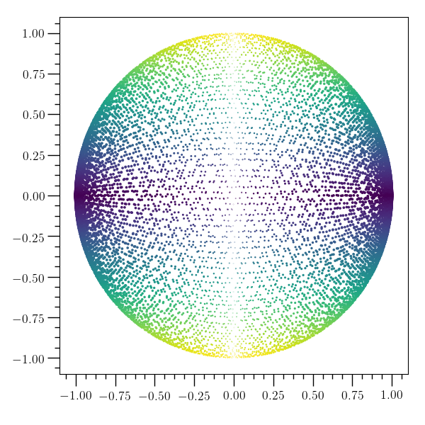
Scatter plot example
# This example demonstrates the use of 'scatter'. It creates a
# circular data set and uses the x value for the size of the points
# and the y value for the color. For no variation in either marker
# size or color, the string 'None' can be used in place of the name of
# the third or fourth column argument to the scatter command.
# For more detail, try e.g. 'o2graph -help table scatter'.
#
o2graph -create table N grid:0,10000,1 \
        -function "sin(1e8*N)" x -function "cos(1.001e8*N)*sqrt(1-x*x)" y \
        -function "4*abs(x)" s -function "abs(y)" c \
        -scatter x y s c -save figures/table_scatter.png
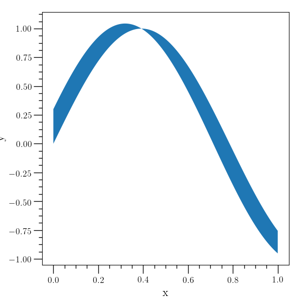
Region plot example
# This example demonstrates the use of 'rplot'. In this case
# the y-axis title is pushed a little too far to the left so
# we increase the left margin before plotting a little bit to compensate.
# For more detail, try e.g. 'o2graph -help table rplot'.
#
o2graph -create table x grid:0,1,1.0e-3 \
        -function "sin(4*x)" y1 \
        -function "sin(4*x)+0.3*cos(4*x)" y2 \
        -xtitle x -ytitle y -set fig_dict "left_margin=0.15" \
        -rplot x y1 x y2 -save figures/table_rplot.png
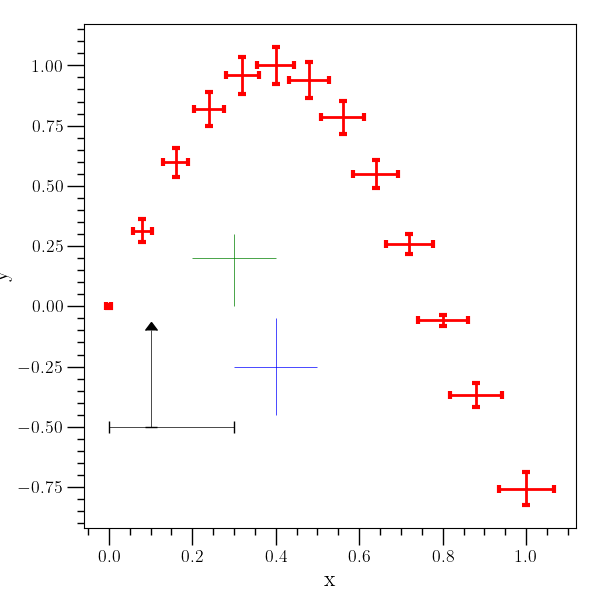
Error bars example
# An example with errorbars. A table is created to demonstrate
# plotting a dataset with error bars (the 'errorbar' command), and
# then three individual points are plotted with error bars (the
# 'error-point' command).
#
o2graph -create table x grid:0,1,8.0e-2 \
        -function "sin(4*x)" y \
        -function "0.06*(sqrt(x)+0.1)" xe \
        -function "0.07*(sqrt(abs(y))+0.1)" ye \
        -xtitle x -ytitle y \
        -errorbar x y xe ye \
        ecolor=red,elinewidth=2,capsize=3,capthick=3,lw=0 \
        -error-point 0.4 "(-0.25)" 0.1 0.2 ecolor=blue \
        -error-point 0.3 0.2 0.1 None 0.2 0.1 ecolor=green \
        -error-point 0.1 "(-0.5)" 0.1 0.2 0.3 0.4 \
        lolims=True,ecolor=black,capsize=4 \
        -save figures/table_errorbar.png
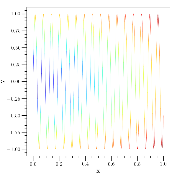
plot-color example
# An example of the 'plot-color' command. The third argument specifies
# the color value and the fourth argument specifies the color map.
# Note that 'plot-color' builds the curve up from line segments, so a
# relatively fine grid is needed to generate this image.
#
o2graph -backend Agg -create table x grid:0,1,0.002 -function "sin(100*x)" y \
-function "sqrt(x^2+y^2)" z -set fig_dict left_margin=0.15 \
-plot-color x y z jet -xtitle x -ytitle y \
-save figures/table_plot_color.png
Modifying axis example
# An example showing how to modify axes using the 'modax' command.
#
o2graph -backend Agg -create table x grid:-3.14,3.14,0.1 \
        -function "(1+sin(x))/2" y \
        -set xlo "(-3.14)" -set xhi 3.14 -xtitle "$ x$" -deriv x y yp \
        -preview 20 -internal data/modax.o2 -plot x y marker=.,color=blue \
        -plot x yp lw=2,color=red -text 0.5 0.95 "$ f(x)$" \
        -text 1 0.05 "$ f^{\prime}(x)$" \
        -modax x_loc=tb,y_minor_loc=0.1,y_tick_dir=inout,labelsize=20 \
        -modax y_tick_len=10,y_minor_tick_len=10 \
        -save figures/modax.png
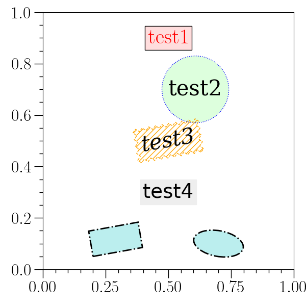
Textbox example
# This example demonstrates the use of 'textbox'.
#
o2graph -backend Agg \
        -set font 30 -textbox 0.5 0.9 test1 fc=#ffdddd color=red \
        -set usetex 0 \
        -textbox 0.5 0.7 test2 fc=#ddffdd,boxstyle=Circle,ec=blue,ls=: \
        fontfamily=serif,ha=left \
        -textbox 0.5 0.5 test3 \
        "fill=False,boxstyle=Sawtooth,ec=orange,ls=--,hatch=///" \
        "fontstyle=italic,rotation=10" \
        -ttext 0.5 0.3 "test4" \
        fontfamily=sans-serif,fontsize=28,backgroundcolor=#eeeeee \
        -rect 0.2 0.05 0.4 0.15 10 \
        fc=#bbeeee,ls=-.,lw=2,ec=black \
        -ellipse 0.7 0.1 0.2 0.1 "(-10)" \
        fc=#bbeeee,ls=-.,lw=2,ec=black \
        -save figures/textbox.png
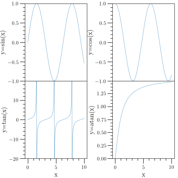
Subplot example 1
# Subplot example with simple 'plot' functions. A two-by-two grid of
# subplots is created, sharing the x-axis between the first and
# second rows, and 'selax' is used to select the subplots.
#
o2graph -backend Agg -create table x func:1001:i/100.0 \
        -function "sin(x)" y1 \
        -function "cos(x)" y2 \
        -function "tan(x)" y3 \
        -function "atan(x)" y4 \
        -subplots 2 2 sharex=True \
        -selax 0 -set ylo "(-1)" -set yhi 1.0 -plot x y1 \
        -ytitle "y=sin(x)" \
        -selax 1 -set ylo "(-1)" -set yhi 1.0 -plot x y2 \
        -ytitle "y=cos(x)" \
        -selax 2 -set ylo "(-20)" -set yhi 19.9 -plot x y3 \
        -xtitle x -ytitle "y=tan(x)" \
        -selax 3 -set ylo "(0)" -set yhi 1.49 -plot x y4 \
        -xtitle x -ytitle "y=atan(x)" \
        -subadj hspace=0,left=0.14,right=0.98,top=0.98,bottom=0.11,wspace=0.41 \
        -save figures/subplots1.png
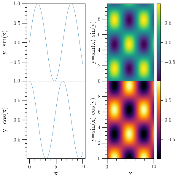
Subplot example 2
# Subplot example mixing 'plot' and 'den-plot' commands, with
# colorbars for the density plots. Setting colorbar to 1 implies that
# all future density plots will contain their own colorbar. The 'eval'
# command can be used to execute python code which isn't easily done
# with o2graph commands. One of the axes is not needed, so the 'eval'
# command is used to make it invisible.
#
o2graph -backend Agg -create table x func:1001:i/100.0 \
        -function "sin(x)" y1 \
        -function "cos(x)" y2 \
        -subplots 2 2 sharex=True \
        -selax 0 -set ylo "(-0.99)" -set yhi 1.0 -plot x y1 \
        -ytitle "y=sin(x)" \
        -selax 2 -set ylo "(-0.99)" -set yhi 1.0 -plot x y2 \
        -ytitle "y=cos(x)" -xtitle x \
        -create table3d x func:1001:i/100.0 y func:1000:i/100.0 \
        z "sin(x)*sin(y)" -function "sin(x)*cos(y)" z2 \
        -set colbar 1 \
        -selax 1 -den-plot z -modax x_visible=False \
        -xtitle x -ytitle "y=sin(x) sin(y)" \
        -selax 3 -set ylo 0 -set yhi 9 -den-plot z2 cmap=inferno \
        -xtitle x -ytitle "y=sin(x) cos(y)" \
        -subadj hspace=0,left=0.15,right=0.93,top=0.98,bottom=0.11,wspace=0.37 \
        -save figures/subplots2.png
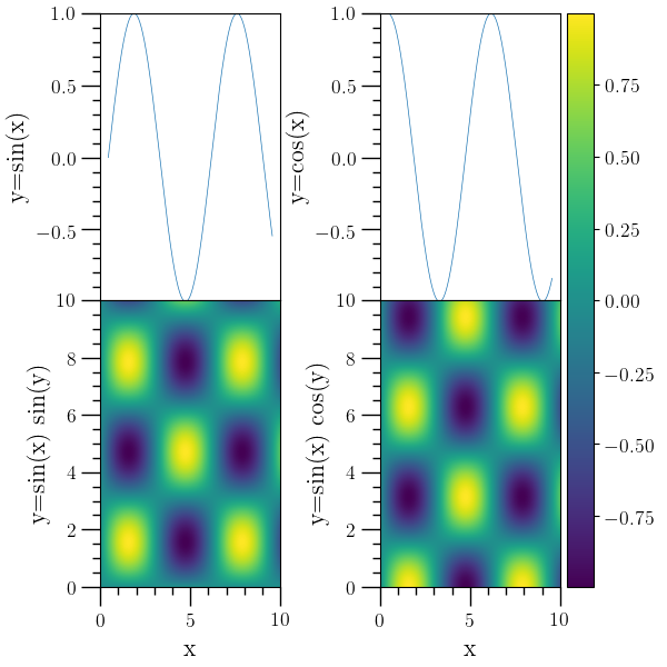
Subplot example 3
# Subplots sharing a colorbar. In this example, the 'addcbar' command
# is used to create a independent color bar based on the last image
# plotted.
#
o2graph -backend Agg -create table x func:1001:i/100.0 \
        -function "sin(x)" y1 \
        -function "cos(x)" y2 \
        -subplots 2 2 sharex=True \
        -subadj hspace=0,left=0.15,right=0.84,top=0.98,bottom=0.12,wspace=0.55 \
        -selax 0 -set ylo "(-0.99)" -set yhi 1.0 -plot x y1 \
        -ytitle "y=sin(x)" \
        -selax 1 -set ylo "(-0.99)" -set yhi 1.0 -plot x y2 \
        -ytitle "y=cos(x)" \
        -create table3d x func:1001:i/100.0 y func:1001:i/100.0 \
        z "sin(x)*sin(y)" -function "sin(x)*cos(y)" z2 \
        -selax 2 -den-plot z \
        -xtitle x -ytitle "y=sin(x) sin(y)" \
        -selax 3 -den-plot z2 \
        -xtitle x -ytitle "y=sin(x) cos(y)" \
        -addcbar 0.85 0.12 0.04 0.86 \
        -selax \
        -save figures/subplots3.png
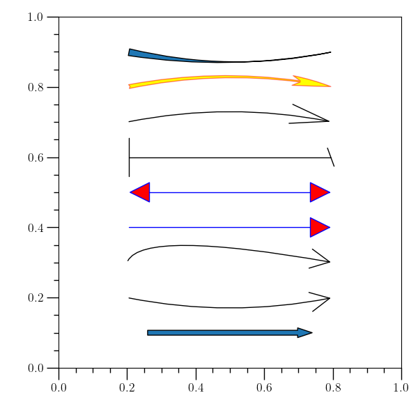
Arrows example
# This example demonstrates the use of 'arrow'.
#
o2graph -backend Agg -xlimits 0 1 -ylimits 0 1.0 \
-arrow 0.2 0.1 0.8 0.1 \
width=5,headwidth=10,headlength=15,shrink=0.1 \
-arrow 0.2 0.2 0.8 0.2 \
arrowstyle='->',connectionstyle=arc3,head_length=2.0,head_width=1.0,rad=0.1 \
-arrow 0.2 0.3 0.8 0.3 \
arrowstyle='->',connectionstyle=angle3,head_length=2.0,head_width=1.0,angleA=70,cs_angleB=170 \
-arrow 0.2 0.4 0.8 0.4 \
arrowstyle='-|>',connectionstyle=arc,fc=red,ec=blue,head_length=2.0,head_width=1.0 \
-arrow 0.2 0.5 0.8 0.5 \
arrowstyle='<|-|>',connectionstyle=arc,fc=red,ec=blue,head_length=2.0,head_width=1.0,lengthA=0.1,lengthB=0.3,angleA=20,as_angleB=20,widthA=20.0,widthB=4 \
-arrow 0.2 0.6 0.8 0.6 \
arrowstyle='|-|',widthA=2.0,as_angleB=20,connectionstyle=arc,angleA=70,cs_angleB=40,rad=0.1 \
-arrow 0.2 0.7 0.8 0.7 \
arrowstyle='->',connectionstyle=arc3,head_length=4.0,head_width=1.0,rad=-0.1 \
-arrow 0.2 0.8 0.8 0.8 \
"arrowstyle=fancy,connectionstyle=arc3,head_length=4.0,head_width=1.0,fc=(1,1,0),ec=[1,0,0,0.5],rad=-0.1" \
-arrow 0.2 0.9 0.8 0.9 \
arrowstyle=wedge,connectionstyle=arc3,tail_width=0.7,shrink_factor=0.1,rad=0.1 \
-save figures/arrows.png
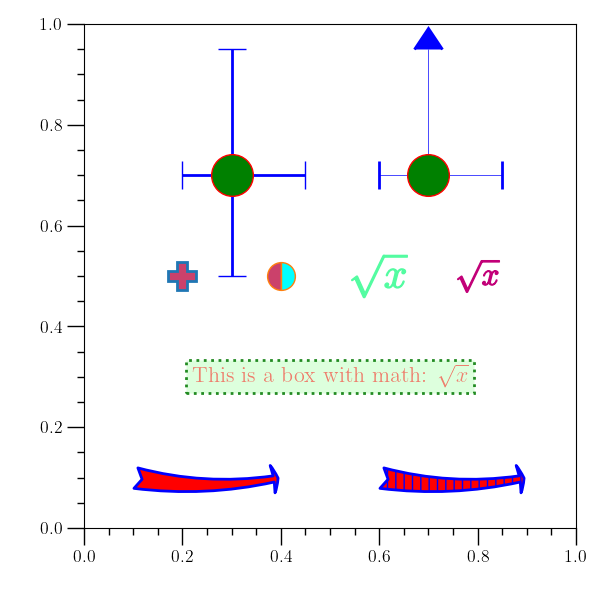
Object properties example
o2graph -backend Agg -xlimits 0 1 -ylimits 0 1 \
-arrow 0.1 0.1 0.4 0.1 \
"arrowstyle=fancy,connectionstyle=arc3,rad=0.1,ec=blue,fc=(1,0,0),lw=2,tail_width=1.5,head_width=2.0" \
-arrow 0.6 0.1 0.9 0.1 \
"arrowstyle=fancy,connectionstyle=arc3,rad=0.1,ec=blue,fc=(1,0,0),lw=2,tail_width=1.5,head_width=2.0,hatch=||" \
-textbox 0.5 0.3 "This is a box with math: $\sqrt{x}$" "fc=#ddffdd,ec=forestgreen,ls=:,lw=2" "color=[1,0,0,0.5]" \
-point 0.2 0.5 "marker=P,ms=20,mfc=xkcd:sea green,mfc=xkcd:dark pink,mew=2" \
-point 0.4 0.5 "marker=o,ms=20,fillstyle=left,mfc=xkcd:sea green,mfc=xkcd:dark pink,mew=1,mfcalt=(0,1,1)" \
-point 0.6 0.5 "marker=$\sqrt{x}$,ms=40,c=xkcd:sea green" \
-point 0.8 0.5 "marker=$\sqrt{x}$,ms=30,c=xkcd:magenta" \
-error-point 0.3 0.7 0.1 0.15 0.2 0.25 \
"marker=o,ms=30,mfc=green,mec=red,ecolor=blue,capsize=10,elinewidth=2" \
-error-point 0.7 0.7 0.1 0.15 0.2 0.25 \
"marker=o,ms=30,mfc=green,mec=red,ecolor=blue,capsize=10,capthick=2,lolims=True" \
-save figures/obj_props.png
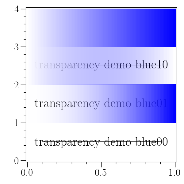
Colormap and transparency example
o2graph -create table3d x grid:0,1,0.01 y grid:0,1,0.01 z x \
-set xlo "(-0.01)" -set xhi 1.01 -set ylo "(-0.04)" -set yhi 4.04 \
-set font 30 \
-ttext 0.5 0.125 "transparency demo blue00" zorder=2 \
-line 0.1 0.5 0.9 0.5 "color=black,zorder=1" \
-cmap blue00 "[1,1,1,0]" "[0,0,1,0]" \
-den-plot z "cmap=blue00,zorder=3" \
-ttext 0.5 0.375 "transparency demo blue01" zorder=2 \
-line 0.1 1.5 0.9 1.5 "color=black,zorder=1" \
-set-grid 1 y+1 \
-cmap blue01 "[1,1,1,0]" "[0,0,1,1]" \
-den-plot z "cmap=blue01,zorder=3" \
-ttext 0.5 0.625 "transparency demo blue10" zorder=2 \
-line 0.1 2.5 0.9 2.5 "color=black,zorder=1" \
-set-grid 1 y+1 \
-cmap blue10 "[1,1,1,1]" "[0,0,1,0]" \
-den-plot z "cmap=blue10,zorder=3" \
-ttext 0.5 0.875 "transparency demo blue11" zorder=2 \
-line 0.1 3.5 0.9 3.5 "color=black,zorder=1" \
-set-grid 1 y+1 \
-cmap blue11 "[1,1,1,1]" "[0,0,1,1]" \
-den-plot z "cmap=blue11,zorder=3" -save figures/cmap_den_plot.png
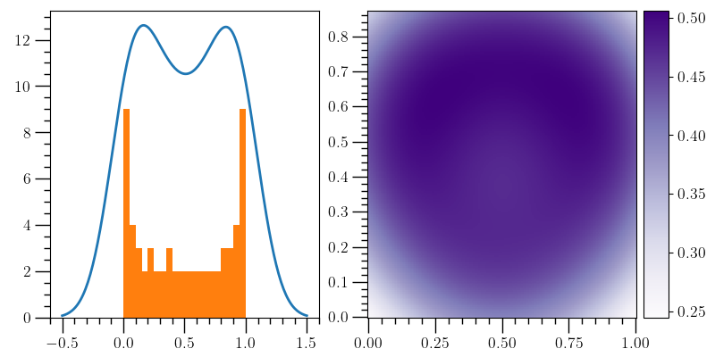
KDE plot example
o2graph -backend Agg -set fig_dict fig_size_x=8,fig_size_y=4 \
        -create table x grid:-3.14,3.14,0.1 \
        -function "(1+sin(x))/2" y \
        -function "(1+cos(x))^(0.8)/2" z \
        -subplots 1 2 -selax 0 -kde-plot \
        y x_min=-0.5,x_max=1.5,y_mult=15,lw=2 \
        -hist-plot y bins=20 -selax 1 \
        -kde-2d-plot y z cmap=Purples -subadj \
        left=0.07,right=0.89,top=0.97,bottom=0.11,wspace=0.18 \
        -addcbar 0.90 0.11 0.035 0.86 \
        -save figures/kde_plot.png
Internal structure
The O2graph script works by creating an instance of the
o2sclpy.o2graph_plotter class and calling the function
o2sclpy.o2graph_plotter.parse_argv() . Internally, the
o2graph_plotter class works by calling the global functions
mentioned in the Python Integration page in the in the O2scl documentation.